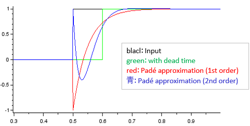
Time delays in control systems create infinite-dimensional transfer functions that severely complicate stability analysis. The 1st order pade approximation directly solves this by converting exponential dead time into a manageable, rational linear expression. By bridging the gap between exact mathematical time-shifting and practical polynomial transfer functions, engineers can easily apply standard tuning rules, Root Locus, and Routh-Hurwitz criteria to delayed systems.
Quick Facts: 1st Order Pade Approximation
- Primary Function: Converts transcendental time delay ($e^{-\theta s}$) into a rational transfer function.
- Mathematical Formula: $e^{-\theta s} \approx \frac{1 – \frac{\theta}{2}s}{1 + \frac{\theta}{2}s}$
- Key Dynamic Introduced: Adds a Right-Half Plane (RHP) zero to the closed-loop system.
- Best Used For: Systems with relatively small dead times (low frequencies).
Why Systems Need the 1st Order Pade Approximation
In continuous time domains, a transport delay (or dead time) of $\theta$ seconds is represented in the Laplace domain as $e^{-\theta s}$. This exponential term cannot be analyzed using standard linear control tools because traditional polynomial structures drive linear system theories. If you attempt to run a closed-loop stability check on $1 + G(s)e^{-\theta s} = 0$, you are faced with an infinite number of roots.
The 1st order pade approximation replaces this problematic exponential with a simple fraction. This transforms a system with an infinite number of states into a standard finite-order model. The resulting approximate model allows you to design PID controllers, assess phase margins, and predict closed-loop performance without relying on highly complex numerical simulations.
The Exact Formula and Derivation
The Padé approximant is a specific type of rational fraction that closely matches a function’s Taylor series expansion up to a given order. For a time delay $\theta$, the basic 1st order pade approximation formula is:
$$e^{-\theta s} \approx \frac{1 – \frac{\theta}{2}s}{1 + \frac{\theta}{2}s}$$
To understand why this specific arrangement works, look at the Taylor series expansion for the exponential function. An exact exponential expands to $1 – \theta s + \frac{(\theta s)^2}{2!} – \dots$. When you perform long division on the 1st order pade approximation fraction, the resulting polynomial perfectly matches the first two terms of the Taylor series while providing mathematically superior stability bounds at higher frequencies.
1st Order Pade Approximation vs. Taylor Series
Engineers frequently ask why they shouldn’t just use a simple truncated Taylor series ($1 – \theta s$) to approximate system delay. The table below outlines why Padé is the industry standard.
| Feature | 1st Order Pade Approximation | Truncated Taylor Series (1−θs) |
| Magnitude Response | Exactly 1 (All-pass behavior). | Approaches infinity as frequency increases. |
| Phase Accuracy | Accurate at low frequencies, bounds strictly. | Highly inaccurate at moderate-to-high frequencies. |
| System Stability | Denominator pole keeps the model stable. | Only features a numerator (zero), distorting stability calculations. |
| Physical Realism | Mimics true time delays realistically. | Creates non-physical amplification of high-frequency noise. |
The Impact of the Right-Half Plane Zero
Applying the 1st order pade approximation mathematically introduces a zero into the Right-Half Plane (RHP) at $s = \frac{2}{\theta}$. This is a critical engineering insight because RHP zeros create non-minimum phase behavior.
When a system features non-minimum phase dynamics, it exhibits an inverse response. If you apply a step input to the system, the initial output will briefly move in the opposite direction of its final steady-state value. By utilizing the 1st order pade approximation, your modeled transfer function accurately captures this initial “wrong-way” behavior, ensuring your controller is tuned to handle the true physical lag of the system.
Practical Applications in Control Theory
Modeling time delays accurately impacts every phase of control system design. Here is how engineers utilize this approximation in real-world workflows:
- PID Controller Tuning: Advanced tuning rules require a rational transfer function. Replacing dead time with this approximation allows you to directly calculate optimal Proportional, Integral, and Derivative gains analytically.
- Root Locus Analysis: Root locus plots require distinct poles and zeros. The approximation supplies a distinct pole at $s = -\frac{2}{\theta}$ and a zero at $s = \frac{2}{\theta}$, enabling accurate visual stability tracking.
- Bode Plot Generation: While exact delays cause continuous phase to drop linearly to negative infinity, the approximated phase drops to a finite limit. This is often sufficient for calculating phase margins securely around the crossover frequency.
Step-by-Step Implementation Example
Let’s apply the 1st order pade approximation to a standard First Order Plus Dead Time (FOPDT) process. Assume a system with a gain of 5, a time constant of 10 seconds, and a dead time of 2 seconds.
The exact transfer function is:
$$G(s) = \frac{5}{10s + 1} e^{-2s}$$
Using the approximation formula for $\theta = 2$:
$$e^{-2s} \approx \frac{1 – s}{1 + s}$$
Substitute this fraction back into the original transfer function:
$$G_{approx}(s) = \left( \frac{5}{10s + 1} \right) \left( \frac{1 – s}{1 + s} \right)$$
Multiply the numerators and denominators to finalize the model:
$$G_{approx}(s) = \frac{5 – 5s}{10s^2 + 11s + 1}$$
You now have a standard second-order transfer function with a RHP zero. You can immediately extract the characteristic equation, check for stability, or input this directly into software for simulation.
Simulating the 1st Order Pade Approximation in MATLAB
Modern control engineers rarely calculate polynomials by hand. MATLAB provides built-in commands to instantly generate the approximation.
Matlab
% Define the time delay
theta = 2;

% Generate the 1st order pade approximation numerator and denominator
[num, den] = pade(theta, 1);

% Create the transfer function block
delay_tf = tf(num, den);
When you link delay_tf in series with your plant model, the step() command will accurately visualize the inverse response caused by the RHP zero. This allows for rapid tuning iteration when testing different delay tolerances.
Common Mistakes When Modeling Dead Time
Even with a reliable mathematical formula, modeling time delay is prone to process errors. Avoid these common pitfalls when applying the 1st order pade approximation to industrial systems:
- Using it for dominant delays: If your dead time is larger than your system’s primary time constant ($\theta > \tau$), a first-order model is generally insufficient. The phase mismatch at lower frequencies will cause your controller to act aggressively, leading to real-world instability.
- Ignoring high-frequency noise: The magnitude of the approximation is exactly 1 at all frequencies. Unlike real physical systems which often attenuate high frequencies, this model passes high-frequency noise perfectly. Always ensure your controller features adequate high-frequency roll-off.
- Cascading approximations incorrectly: Do not string together multiple 1st order pade approximation blocks to simulate a larger aggregated delay. This creates an unnecessary number of RHP zeros that mathematically distort the system matrix.
When to Move Beyond the 1st Order Pade Approximation
The 1st order pade approximation is a foundational tool, but it possesses strict bandwidth limitations. The approximation holds true mathematically only when $\theta \omega < 1$ (where $\omega$ is the frequency in radians per second).
If your system operates near or above this threshold, or if highly aggressive closed-loop control is required, you must upgrade to a 2nd or 3rd order Padé model. A 2nd order approximation introduces complex conjugate poles and zeros, providing a significantly tighter phase match at higher frequencies. However, this comes at the cost of algebraic complexity, often necessitating software-driven analysis rather than simple hand calculations.
Mastering the 1st order pade approximation gives engineers a direct, reliable bridge between infinite-dimensional reality and finite-dimensional mathematics. By understanding the formula’s structural origin, leveraging its all-pass magnitude, and respecting the hard limits of its phase accuracy, you can build highly robust control architectures. Whether you are stabilizing a chemical reactor’s transport feed or compensating for digital network latency, this approximation remains one of the most practical and vital techniques utilized in modern control engineering.